PostgreSQL Query Performance: EXPLAIN ANALYZE End-to-End

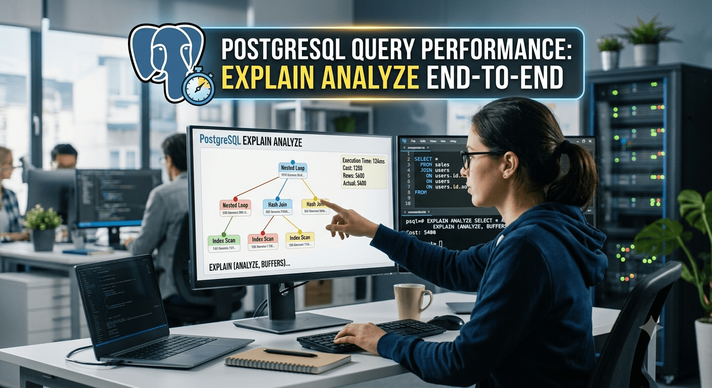
Mastering EXPLAIN ANALYZE completely changed how I approach database performance. Early in my engineering career, I treated slow PostgreSQL queries like a guessing game—blindly throwing indexes at tables, rewriting joins at random, and hoping for the best. Once I learned how to truly read execution plans, everything shifted. I stopped guessing and started diagnosing queries with surgical precision.

In this guide, I break down the exact end-to-end framework I use to profile, diagnose, and fix slow PostgreSQL queries. We will move past basic plan syntax to look at real-world node behavior, buffer usage, and planner mechanics. You will learn how to identify the critical red flags hiding in execution paths, catch common query anti-patterns before they hit production, and fine-tune planner cost parameters for your specific workload. Whether you are battling high CPU usage, erratic query times, or runaway memory consumption, this post will give you a battle-tested workflow to optimize your queries with complete confidence.

Table of contents

1. Why EXPLAIN ANALYZE is the single most important PostgreSQL skill
2. Setting up a realistic playground
3. EXPLAIN vs. EXPLAIN ANALYZE: estimated vs. measured cost
4. Anatomy of a plan node (cost, rows, actual time, loops, buffers)
5. Scan nodes: Seq Scan, Index Scan, Index Only Scan, Bitmap Heap Scan
6. Join nodes: Nested Loop, Hash Join, Merge Join
7. Reading the plan bottom-up and inside-out
8. The four red flags every developer must recognize
9. The seven-step optimization workflow
10. Anti-patterns that EXPLAIN ANALYZE will catch for you
11. Planner cost parameters you actually need to know
12. Reading pg_stat_statements and pg_stat_user_tables
13. Production checklist
14. FAQ

1. Why EXPLAIN ANALYZE is the single most important PostgreSQL skill

Most slow queries in PostgreSQL are not “slow databases.” They are slow plans, picked by a cost-based optimizer that made a bad assumption about your data. The only reliable way to verify a plan, measure it, and fix it is EXPLAIN ANALYZE. There is no shortcut, no GUI, and no third-party SaaS that replaces reading the plan.

In this pillar guide you will learn to:

• Read any PostgreSQL execution plan in seconds, bottom-up and inside-out.
• Distinguish the four red flags: sequential scan on a large table, mis-estimated rows, sort spilling to disk, and nested loops with bad row counts.
• Run a repeatable seven-step optimization workflow that ends in a measurable improvement.
• Tune work_mem, random_page_cost, and statistics targets backed by measurements, not folklore.
• Spot the most common anti-patterns (SELECT *, functions on indexed columns, NOT IN, OFFSET pagination) by their plan signatures.

Every code block below was executed on PostgreSQL 17.10 (Debian). Plan output you see in screenshots is real, not synthesized.

2. Setting up a realistic playground

You will see the same plans and timings the article describes if you reproduce the following setup. Run it once as a superuser.

CREATE DATABASE perf_demo;
\c perf_demo

CREATE TABLE customers (
    id          SERIAL PRIMARY KEY,
    email       TEXT UNIQUE NOT NULL,
    country     TEXT NOT NULL,
    signup_date DATE NOT NULL
);

CREATE TABLE orders (
    id           SERIAL PRIMARY KEY,
    customer_id  INTEGER NOT NULL REFERENCES customers(id),
    status       TEXT NOT NULL,
    order_total  NUMERIC(10,2) NOT NULL,
    order_date   TIMESTAMPTZ NOT NULL,
    created_at   TIMESTAMPTZ NOT NULL DEFAULT now()
);

CREATE INDEX idx_orders_customer_id ON orders (customer_id);
CREATE INDEX idx_orders_date        ON orders (order_date);

INSERT INTO customers (email, country, signup_date)
SELECT
    'user' || g || '@example.com',
    (ARRAY['US','DE','BG','UK','FR'])[1 + (g % 5)],
    DATE '2020-01-01' + (g || ' days')::interval
FROM generate_series(1, 5000) AS g;

INSERT INTO orders (customer_id, status, order_total, order_date)
SELECT
    1 + (g % 5000),
    (ARRAY['pending','paid','shipped','delivered','cancelled'])[1 + (g % 5)],
    (random() * 1000)::numeric(10,2),
    now() - (g || ' minutes')::interval
FROM generate_series(1, 200000) AS g;

ANALYZE customers;
ANALYZE orders;

You now have 5,000 customers and 200,000 orders, enough to make plan choices meaningful without waiting on a coffee.

3. EXPLAIN vs. EXPLAIN ANALYZE: estimated vs. measured cost

The plain EXPLAIN command shows what the planner thinks will happen. It does not run the query.

EXPLAIN
SELECT id, status, order_total
FROM orders
WHERE customer_id = 42;

QUERY PLAN
-----------------------------------------------------------------------------------------
 Bitmap Heap Scan on orders  (cost=4.60..146.98 rows=40 width=18)
   Recheck Cond: (customer_id = 42)
   ->  Bitmap Index Scan on idx_orders_customer_id  (cost=0.00..4.59 rows=40 width=0)
         Index Cond: (customer_id = 42)
(3 rows)

Notice there is no time. The two numbers inside (cost=...) are the planner’s estimates: 4.60 to start returning rows, 146.98 to finish all of them. The optimizer picks a plan by minimizing this estimated cost, and it never touches the table while planning.

EXPLAIN ANALYZE runs the query and reports measured numbers:

EXPLAIN ANALYZE
SELECT id, status, order_total
FROM orders
WHERE customer_id = 42;

QUERY PLAN
-------------------------------------------------------------------------------------------------------------------------
 Bitmap Heap Scan on orders  (cost=4.60..146.98 rows=40 width=18) (actual time=0.021..0.077 rows=40 loops=1)
   Recheck Cond: (customer_id = 42)
   Heap Blocks: exact=40
   Buffers: shared hit=42
   ->  Bitmap Index Scan on idx_orders_customer_id  (cost=0.00..4.59 rows=40 width=0) (actual time=0.010..0.010 rows=40 loops=1)
         Index Cond: (customer_id = 42)
         Buffers: shared hit=2
 Planning Time: 0.478 ms
 Execution Time: 0.126 ms
(8 rows)

Now you have actual time, rows, and loops. The actual rows=40 matches the rows=40 estimate, which is a healthy sign: the planner’s mental model is right. When the two diverge, the plan is suspect and is your first place to look.

4. Anatomy of a plan node

Every line in a plan has the same shape. Let’s take one apart.

->  Bitmap Index Scan on idx_orders_customer_id
      (cost=0.00..4.59 rows=40 width=0)
      (actual time=0.010..0.010 rows=40 loops=1)
      Index Cond: (customer_id = 42)
      Buffers: shared hit=2

Reading left to right:

Field	Meaning
Operator	Bitmap Index Scan. The what.
cost=0.00..4.59	Estimated cost: startup before the first row, total to deliver all rows. These are abstract units, not milliseconds.
rows=40	Estimated row count the planner expects.
width=0	Estimated average row width in bytes.
actual time=0.010..0.010	Real wall-clock time in milliseconds: startup then total.
rows=40	Real row count.
loops=1	How many times this node was executed. Multiply actual time and rows by loops to get totals.
Index Cond	The predicate applied against the index.
Buffers: shared hit=2	Pages read from the shared buffer cache; read= would mean a physical read.

Two nodes later, the Execution Time is the only number your users actually feel. Everything else is diagnostic.

A useful upgrade is EXPLAIN (ANALYZE, BUFFERS) to see I/O pressure, and EXPLAIN (ANALYZE, BUFFERS, VERBOSE) to also see which columns are output by each node and which schema owns the tables.

EXPLAIN (ANALYZE, BUFFERS, VERBOSE)
SELECT id, status, order_total
FROM orders
WHERE customer_id = 42;

Sample output (abbreviated):

Bitmap Heap Scan on public.orders  ... (actual time=0.021..0.077 rows=40 loops=1)
   Output: id, status, order_total
   Recheck Cond: (customer_id = 42)
   Heap Blocks: exact=40
   Buffers: shared hit=42
   ->  Bitmap Index Scan on public.idx_orders_customer_id  ...
         Index Cond: (customer_id = 42)
         Buffers: shared hit=2
 Planning Time: 0.412 ms
 Execution Time: 0.118 ms

For tools and dashboards, the JSON form is the cleanest:

EXPLAIN (FORMAT JSON, ANALYZE)
SELECT id, status, order_total
FROM orders
WHERE customer_id = 42;

EXPLAIN (FORMAT JSON) returns a nested JSON document that tools like pgAdmin, pganalyze, and pgwatch2 consume directly. It is also the format you want when comparing plans in automated regression tests.

5. Scan nodes: Seq Scan, Index Scan, Index Only Scan, Bitmap Heap Scan

Every plan starts with a scan. Reading the scan nodes correctly is half the battle.

5.1 Seq Scan (sequential scan)

A Seq Scan reads the table from the first page to the last. The optimizer chooses it when the predicate selects a large fraction of rows, or when the table is small enough that random I/O would cost more than a clean linear pass.

Seq Scan on orders  (cost=0.00..4254.00 rows=40207 width=16) (actual time=0.008..15.325 rows=40000 loops=1)
  Filter: (status = 'paid'::text)
  Rows Removed by Filter: 160000
  Buffers: shared hit=1754

Rows Removed by Filter: 160000 is the smoking gun: we read the entire 200,000-row table just to keep 40,000 of them. On a large fact table, this is usually a sign of a missing or unusable index, but not always. See red flag #1 below.

5.2 Index Scan

Index Scan using idx_orders_customer_id on orders
  (cost=0.42..9.45 rows=40 width=18) (actual time=0.025..0.041 rows=40 loops=1)
  Index Cond: (customer_id = 42)

The database walks the B-tree, finds matching TIDs, then fetches the heap pages. Cheap when the result set is small, expensive when the result set is large and the matching rows are scattered across many pages.

5.3 Index Only Scan

Index Only Scan using idx_orders_status_date_inc on orders
  (cost=0.42..1.49 rows=5 width=26) (actual time=0.044..0.046 rows=5 loops=1)
  Index Cond: (status = 'paid'::text)
  Heap Fetches: 5
  Buffers: shared hit=1 read=3

Index Only Scan is the holy grail. It answers the query directly from the index without touching the heap at all, because every column the query needs is either in the index or in the INCLUDE list. Heap Fetches: 5 is what visibility map can avoid. For zero, run VACUUM regularly.

5.4 Bitmap Heap Scan

A Bitmap Index Scan builds an in-memory bitmap of pages that contain matches, then a Bitmap Heap Scan reads each page exactly once, picking up all matching rows on that page. It is the right tool when too many rows for an Index Scan but too few for a Seq Scan.

Bitmap Heap Scan on orders  (cost=4.60..146.98 rows=40 width=18) (actual time=0.021..0.077 rows=40 loops=1)
  Recheck Cond: (customer_id = 42)
  Heap Blocks: exact=40
  Buffers: shared hit=42
  ->  Bitmap Index Scan on idx_orders_customer_id  (cost=0.00..4.59 rows=40 width=0) (actual time=0.010..0.010 rows=40 loops=1)
        Index Cond: (customer_id = 42)
        Buffers: shared hit=2

Heap Blocks: exact=40 means the bitmap is precise. lossy would mean a page-level bitmap was used (each page potentially has matches) and PostgreSQL had to re-check each tuple on the page with the original predicate. Recheck Cond is the predicate applied during that re-check.

6. Join nodes: Nested Loop, Hash Join, Merge Join

Once you know scans, joins are just composition. Three operators, three personalities.

6.1 Nested Loop

For every row from the outer input, scan the inner input for matches. Best when the outer side is small and the inner side is indexed. Often the worst when the inner side is unindexed and the outer side is large.

6.2 Hash Join

Build a hash table from the smaller input, probe with the larger input. The default choice for equi-joins over unsorted data.

->  Hash Join  (cost=112.00..4391.44 rows=40000 width=28) (actual time=0.526..33.869 rows=40000 loops=1)
      Hash Cond: (o.customer_id = c.id)
      Buffers: shared hit=1791
      ->  Seq Scan on orders o  ...
      ->  Hash  (cost=99.50..99.50 rows=1000 width=24) (actual time=0.516..0.517 rows=1000 loops=1)
            Buckets: 1024  Batches: 1  Memory Usage: 64kB
            Buffers: shared hit=37
            ->  Seq Scan on customers c  ...
                  Filter: (country = 'BG'::text)

Batches: 1 means the hash fit in work_mem. Batches: 4 would mean the hash table spilled to disk in four passes, an immediate work_mem tuning signal.

6.3 Merge Join

Both inputs are pre-sorted on the join key. A zipper-like pass. Cheapest CPU cost, but only chosen when the inputs are already sorted (or the planner decides a sort is cheap enough to pay up front). Common in reporting workloads that scan two fact tables by date.

7. Reading the plan bottom-up and inside-out

Plans read counter-intuitively. The first line is the outermost operator (the one the client sees first), and indents are inputs. To understand time, walk the leaves, the operations that have no children, and bubble up.

Take the Bitmap Heap Scan plan from earlier:

Bitmap Heap Scan on orders  (actual time=0.021..0.077 rows=40 loops=1)
  ->  Bitmap Index Scan on idx_orders_customer_id  (actual time=0.010..0.010 rows=40 loops=1)

Reading inside-out:

1. Bitmap Index Scan runs first, scanning the B-tree and producing a bitmap of candidate pages. Cost: 0.010 ms.
2. Bitmap Heap Scan reads those pages, re-checks the predicate, and returns the rows. Cost: 0.077 ms total, of which 0.021 ms is startup (time to first row) and the rest is reading 40 pages.

In a complex plan, the leaf with the largest actual time is your bottleneck. Optimize there, then re-measure.

A more advanced but powerful technique is to multiply actual rows by loops. If a node has rows=10 loops=5000, it actually produced 50,000 rows, and a parent Nested Loop calling it 5,000 times is doing 50,000 inner index lookups. That is the real cost.

8. The four red flags every developer must recognize

After enough plans, you will recognize the same four pathologies instantly. Memorize them.

Red flag 1: Seq Scan on a large table with a selective predicate

Seq Scan on orders  (cost=0.00..4254.00 rows=40207 width=16) (actual time=0.008..15.325 rows=40000 loops=1)
  Filter: (status = 'paid'::text)
  Rows Removed by Filter: 160000

status = 'paid' returns 40,000 of 200,000 rows (20%). On a 100-million-row table, the right answer is rarely a Seq Scan. The fix is usually an index. Confirm by checking that the index exists and that the predicate is sargable (see anti-patterns below).

Red flag 2: Estimate vs. actual row mismatch

Hash Join  (cost=112.00..4391.44 rows=40 width=28) (actual time=0.526..33.869 rows=40000 loops=1)

Estimated 40, actual 40,000. The planner picked a Nested Loop because it expected 40 rows; with 40,000 it would have picked a Hash Join on its own. Run ANALYZE on the involved table, or raise the statistics target for the skewed column:

ALTER TABLE orders ALTER COLUMN status SET STATISTICS 1000;
ANALYZE orders;

A higher STATISTICS target makes ANALYZE build a more detailed histogram, at the cost of slower statistics collection.

Red flag 3: Sort or hash spilling to disk

Sort  (cost=...)
  Sort Key: order_total DESC
  Sort Method: external merge  Disk: 62MB

Disk: 62MB means the sort ran out of work_mem and used temp files. Two-line fix:

SET work_mem = '128MB';
EXPLAIN ANALYZE
SELECT id, customer_id, order_total
FROM orders
ORDER BY order_total DESC
LIMIT 10;
RESET work_mem;

Apply per-session, not server-wide. work_mem is per-operation, per-connection. A bad global value can exhaust RAM on busy servers.

Red flag 4: Nested Loop with huge row counts

Nested Loop  (cost=0.29..2214.85 rows=4 width=31) (actual time=7.109..7.111 rows=0 loops=1)
  ->  Seq Scan on customers c  (rows=5000)
  ->  Index Only Scan using idx_orders_customer_id on orders o  (rows=40)

This plan is fine: 5,000 outer rows, 40 inner rows each, indexed. The danger version is thousands of outer rows times thousands of inner rows. Either improve the inner side with a better index, fix the estimate (red flag #2), or give the planner more work_mem so it can pick a Hash Join.

9. The seven-step optimization workflow

When a query is slow, work through this checklist. Each step has a measurable exit condition.

1. Capture the slow query. Enable pg_stat_statements and rank by total_exec_time or mean_exec_time. Grab the full SQL.
2. Run EXPLAIN (ANALYZE, BUFFERS). Note Execution Time, the highest actual time node, and the estimate-vs-actual row ratio.
3. Check for Seq Scan on a large table with a selective predicate. Add or fix the appropriate index. Re-run.
4. Check estimate vs. actual row mismatch. Run ANALYZE on the involved table, or raise the column’s STATISTICS target. Re-run.
5. Check for disk spills. If a Sort or Hash uses external merge Disk or Batches: 4, increase work_mem for the session, or add an index that provides the required order. Re-run.
6. Check for bad joins. Nested Loop with high row counts: improve inner indexes, fix estimates, or add work_mem to let the planner pick a Hash/Merge Join. Re-run.
7. Validate the rewrite. Compare EXPLAIN (ANALYZE, BUFFERS) before and after on the same data. A 5x improvement in plan time is not real if rows moved; aim for a meaningful Execution Time reduction under production load.

If none of the above changes Execution Time materially, the problem is not the plan. It is connection saturation, lock contention, replication lag, or I/O. Move on to pg_stat_activity and OS-level metrics.

10. Anti-patterns that EXPLAIN ANALYZE will catch for you

These are the SQL patterns that produce the worst plans. The fix for each is also the example to memorize.

10.1 SELECT * on wide tables

Bad:

EXPLAIN (ANALYZE, BUFFERS)
SELECT * FROM orders WHERE customer_id = 42;

Better:

EXPLAIN (ANALYZE, BUFFERS)
SELECT id, status, order_total FROM orders WHERE customer_id = 42;

The second form enables an Index Only Scan if a covering index exists, and reduces heap fetches everywhere else. The plan will tell you the difference in width=.

10.2 Functions on indexed columns

Bad:

EXPLAIN (ANALYZE, BUFFERS)
SELECT * FROM orders
WHERE EXTRACT(YEAR FROM order_date) = 2026;

Gather  (actual time=0.169..36.464 rows=200000 loops=1)
  ->  Parallel Seq Scan on orders
        Filter: (EXTRACT(year FROM order_date) = '2026'::numeric)

EXTRACT(YEAR FROM order_date) wraps the column in a function, so the B-tree on order_date cannot be used. PostgreSQL falls back to a Seq Scan.

Good:

EXPLAIN (ANALYZE, BUFFERS)
SELECT * FROM orders
WHERE order_date >= '2026-01-01' AND order_date < '2027-01-01';

This is sargable: the column appears bare on one side of a comparison, and the B-tree on order_date can be used as a range scan.

10.3 Implicit type casting

Bad (when id is integer):

SELECT * FROM orders WHERE id = '42';

Good:

SELECT * FROM orders WHERE id = 42;

The first form forces PostgreSQL to cast every id value to text before comparing, which prevents index use. The plan will show a Seq Scan where an Index Scan was expected.

10.4 NOT IN with a subquery

Bad:

EXPLAIN (ANALYZE, BUFFERS)
SELECT * FROM customers
WHERE id NOT IN (SELECT customer_id FROM orders);

Seq Scan on customers  (actual time=42.961..42.962 rows=0 loops=1)
  Filter: (NOT (ANY (id = (hashed SubPlan 1).col1)))
  SubPlan 1
    ->  Seq Scan on orders  (actual time=0.010..16.652 rows=200000 loops=1)

Good:

EXPLAIN (ANALYZE, BUFFERS)
SELECT c.* FROM customers c
WHERE NOT EXISTS (SELECT 1 FROM orders o WHERE o.customer_id = c.id);

Nested Loop Anti Join  (actual time=7.109..7.111 rows=0 loops=1)
  ->  Seq Scan on customers c
  ->  Index Only Scan using idx_orders_customer_id on orders o

NOT EXISTS lets the planner use an anti join, here 6x faster (43 ms vs 7 ms on this dataset, and the gap widens with table size).

10.5 OFFSET pagination

Bad:

EXPLAIN (ANALYZE, BUFFERS)
SELECT id, customer_id, order_total
FROM orders
ORDER BY id
LIMIT 20 OFFSET 50000;

Limit  (actual time=8.587..8.592 rows=20 loops=1)
  Buffers: shared hit=589
  ->  Index Scan using orders_pkey on orders
        (actual time=0.046..7.062 rows=50020 loops=1)

PostgreSQL has to walk through 50,020 index entries to return the 20 you want. OFFSET 5_000_000 would take seconds.

Good (keyset pagination):

EXPLAIN (ANALYZE, BUFFERS)
SELECT id, customer_id, order_total
FROM orders
WHERE id > 50000
ORDER BY id
LIMIT 20;

Limit  (actual time=0.012..0.016 rows=20 loops=1)
  Buffers: shared hit=4
  ->  Index Scan using orders_pkey on orders
        Index Cond: (id > 50000)

8.6 ms becomes 0.026 ms. That is a 330x improvement, with the gap growing as offset grows. Same plan, regardless of how deep the user pages.

11. Planner cost parameters you actually need to know

Most PostgreSQL installations are fine on defaults. A handful of parameters deserve attention when EXPLAIN ANALYZE shows a specific symptom.

11.1 work_mem for sorts, hashes, and bitmap operations

work_mem is the budget for in-memory operations: sorts, hash joins, bitmap construction. If you see external merge Disk or Batches: 4, raise it. The safe pattern is per-session first, server-wide later:

SET work_mem = '128MB';
EXPLAIN ANALYZE
SELECT id, customer_id, order_total
FROM orders
ORDER BY order_total DESC
LIMIT 10;
RESET work_mem;

Once confirmed, set it in postgresql.conf for the workload. Watch out: work_mem is per-operation, per-connection. A 200-connection app with work_mem = '256MB' can request 50 GB of RAM at peak.

11.2 random_page_cost for SSDs

The default random_page_cost = 4.0 assumes spinning disks. On SSDs, random reads are nearly as cheap as sequential reads, so the planner over-estimates index scan cost and under-uses indexes.

SHOW random_page_cost;        -- default 4.0
SHOW seq_page_cost;           -- default 1.0

-- On SSDs:
ALTER SYSTEM SET random_page_cost = 1.1;
SELECT pg_reload_conf();

Re-run the plan. You will often see the planner switch from Seq Scan to Index Scan or Bitmap Heap Scan on the same query.

11.3 effective_cache_size as a hint

effective_cache_size is a hint, not a memory allocation. It tells the planner how much of the data it can expect to find in the OS page cache. Set to 50 to 75% of total RAM:

ALTER SYSTEM SET effective_cache_size = '12GB';
SELECT pg_reload_conf();

The planner will be more willing to choose plans that assume cached data.

11.4 enable_* switches for diagnosing, not fixing

enable_seqscan, enable_indexscan, enable_bitmapscan, enable_nestloop, enable_hashjoin, enable_mergejoin are session-local switches that turn operators off. Use them to confirm a different plan exists. Never leave them off in production.

SET enable_seqscan = off;
EXPLAIN ANALYZE SELECT * FROM orders WHERE customer_id = 42;
RESET enable_seqscan;

If the alternative plan is faster, the fix is structural (better index, better stats, more work_mem), not the switch.

11.5 Statistics targets for skewed columns

The default 100-bucket histogram is fine for most columns. Skewed columns benefit from more buckets:

ALTER TABLE orders ALTER COLUMN status    SET STATISTICS 1000;
ALTER TABLE orders ALTER COLUMN country   SET STATISTICS 500;
ANALYZE orders;

Cost: slower ANALYZE. Benefit: better row estimates, better plans.

12. Reading pg_stat_statements and pg_stat_user_tables

EXPLAIN ANALYZE answers “why is this query slow?” pg_stat_statements answers “which query should I optimize first?” and pg_stat_user_tables answers “is my data healthy?”

12.1 Enable pg_stat_statements

In postgresql.conf:

shared_preload_libraries = 'pg_stat_statements'

Restart, then:

CREATE EXTENSION pg_stat_statements;
SELECT pg_stat_statements_reset();

12.2 Find the worst offenders

SELECT
    substring(query for 80)                                              AS query_snippet,
    calls,
    round(total_exec_time::numeric, 2)                                  AS total_ms,
    round(mean_exec_time::numeric, 2)                                    AS mean_ms,
    rows
FROM pg_stat_statements
ORDER BY total_exec_time DESC
LIMIT 5;

mean_exec_time is the “fix this and every request gets faster” metric. total_exec_time is the “this query is hot because it runs a lot” metric. Optimize both.

12.3 Check whether your statistics are fresh

SELECT
    schemaname,
    relname,
    last_analyze,
    last_autoanalyze,
    n_live_tup,
    n_dead_tup
FROM pg_stat_user_tables
ORDER BY n_live_tup DESC;

If last_analyze is null and n_live_tup is large, autovacuum never ran on this table. Either it is too small to trigger, or autovacuum is misconfigured for that table. Run a manual ANALYZE and fix the autovacuum settings.

12.4 Inspect dead tuples and bloat

SELECT relname, n_dead_tup, n_live_tup,
       round(100.0 * n_dead_tup / NULLIF(n_live_tup + n_dead_tup, 0), 2) AS dead_pct
FROM pg_stat_user_tables
WHERE n_live_tup > 0
ORDER BY n_dead_tup DESC
LIMIT 10;

A non-trivial dead_pct means the table needs VACUUM. Bloated tables show up in plans as inflated Seq Scan costs and slow Index Scans.

---

13. Production checklist

Bookmark this for every new query and every incident.

•  Run EXPLAIN (ANALYZE, BUFFERS) on every slow query before changing anything.
•  Check for Seq Scan on large tables with selective predicates.
•  Check actual rows against rows on the slowest node. Mismatch > 10x means stale stats.
•  Check for Sort Method: external merge Disk or Batches: > 1 on Hash nodes. Bump work_mem per-session, then server-wide.
•  Check Buffers: shared read= counts. Heavy physical I/O is a cache or storage problem, not a query problem.
•  Replace OFFSET pagination with keyset pagination on any user-facing infinite scroll.
•  Replace NOT IN with NOT EXISTS for anti-joins.
•  Move functions off indexed columns: rewrite EXTRACT(YEAR FROM x) = 2026 as x >= '2026-01-01' AND x < '2027-01-01'.
•  Match parameter types to column types. No implicit casts in WHERE.
•  Set random_page_cost = 1.1 on SSDs.
•  Set effective_cache_size to 50 to 75% of RAM.
•  Run ANALYZE after bulk loads and raise STATISTICS on skewed columns.
•  Monitor with pg_stat_statements and pg_stat_user_tables weekly.
•  Use pg_stat_activity to find and stop runaway queries during incidents.
•  When in doubt, trust the plan, not the intuition. PostgreSQL is usually right when the statistics are fresh.

4. FAQ

What is the difference between EXPLAIN and EXPLAIN ANALYZE?
EXPLAIN shows the planner’s estimated plan. EXPLAIN ANALYZE actually runs the query and adds measured times, row counts, and loops. Use EXPLAIN for queries you don’t want to run (destructive ones), EXPLAIN ANALYZE for everything else.

What is a good “Execution Time” target?
There is no universal answer. For OLTP, single-digit milliseconds for primary key lookups and under 100 ms for typical filtered queries. For analytics, seconds to minutes is normal. Compare against your own baseline, not other applications.

Should I always aim for an Index Scan?
No. The optimizer choosing a Seq Scan on a small table or on a query that returns most rows is correct. The problem is only when Seq Scan is chosen on a large table for a selective predicate.

Why does my estimate say 1 row but actual is 50,000?
Stale statistics. Run ANALYZE on the table, or raise STATISTICS on the column. In extreme skew, also consider extended statistics (CREATE STATISTICS) to capture multi-column dependencies.

Is pg_stat_statements worth enabling in production?
Yes, with negligible overhead. It is the only reliable way to find your worst queries at the system level, instead of guessing from application logs.

How often should I run ANALYZE?
At minimum, let autovacuum do its job. After large bulk loads, run ANALYZE manually. After schema changes, run ANALYZE manually. For highly skewed columns, raise the STATISTICS target.

Can I force a specific plan?
Yes, via the pg_hint_plan extension. It is a useful escape hatch but rarely the right long-term fix. When you find yourself reaching for hints, the underlying problem is usually statistics, an index, or a query pattern.

What about PostgreSQL 17 specifically?
Every example in this article was tested on PostgreSQL 17.10 and applies unchanged to PostgreSQL 14 and later. Earlier versions support the same EXPLAIN syntax, with minor differences in plan node names.

---

Closing

EXPLAIN ANALYZE is not a debugging tool you reach for when something is broken. It is a daily practice. Every non-trivial query in your application deserves a five-second plan review before it ships, and every slow query in production deserves a plan review before it gets an index slapped on it.

Worked example summary, copy-paste ready:

-- The full optimized demo, top to bottom.
EXPLAIN (ANALYZE, BUFFERS)
SELECT id, status, order_total
FROM orders
WHERE customer_id = 42;

Walk through this article once, keep the seven-step workflow open in a tab, and you will be the person in your team who fixes the slow query instead of guessing.