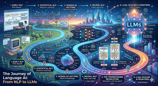
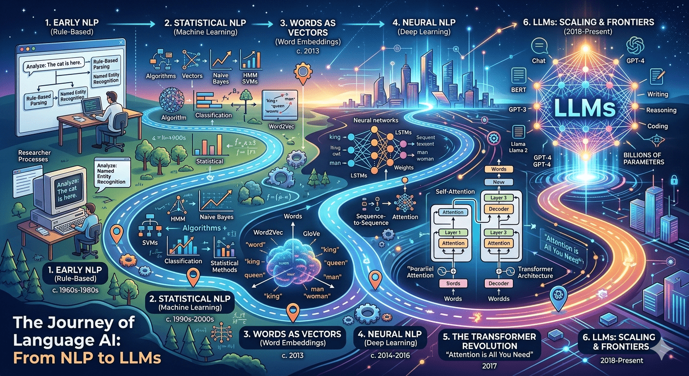
The journey from NLP to LLMs is one of the most fascinating stories in artificial intelligence. In just a few decades, we’ve gone from simple rule-based systems that could barely parse a sentence to models like GPT-4, Claude, and LLaMA that can write essays, generate code, and hold nuanced conversations.
But how did we get here? What are the key concepts, breakthroughs, and technologies that made this possible?
In this article, we’ll walk through the entire evolution of language AI — from classical NLP techniques to modern Large Language Models. Every concept will be explained in simple, accessible terms and accompanied by practical code examples in Python and PyTorch.
Whether you’re a beginner curious about AI or a developer looking to deepen your understanding, this guide will give you a solid foundation.
Table of Contents
- What is Natural Language Processing (NLP)?
- Text Preprocessing: The Foundation
- Bag of Words and TF-IDF
- Word Embeddings: Words as Vectors
- Recurrent Neural Networks (RNNs)
- The Attention Mechanism: A Game Changer
- The Transformer Architecture
- Large Language Models (LLMs)
- Building a Mini LLM from Scratch
- Fine-Tuning Pre-trained LLMs
- The Future of LLMs
- Conclusion
1. What is Natural Language Processing (NLP)?
Natural Language Processing (NLP) is a branch of artificial intelligence that focuses on enabling computers to understand, interpret, and generate human language. It sits at the intersection of computer science, linguistics, and machine learning.
Why is NLP Important?
Every day, humans produce enormous amounts of text data — emails, tweets, articles, reviews, and messages. NLP provides the tools to make sense of all that unstructured data.
Common NLP Tasks
- Sentiment Analysis — Is this review positive or negative?
- Named Entity Recognition (NER) — Identify names, places, and organizations in text.
- Machine Translation — Translate text from one language to another.
- Text Summarization — Condense a long document into key points.
- Question Answering — Given a question, find or generate the answer.
- Text Generation — Produce coherent, human-like text.
A Simple NLP Example with Python
Let’s start with the basics — tokenization, which is the process of breaking text into individual units (tokens):
# Simple tokenization example
text = "Natural Language Processing is fascinating!"

# Basic whitespace tokenization
tokens = text.split()
print("Tokens:", tokens)
# Output: ['Natural', 'Language', 'Processing', 'is', 'fascinating!']

# Using NLTK for more sophisticated tokenization
import nltk
nltk.download('punkt')
from nltk.tokenize import word_tokenize

tokens = word_tokenize(text)
print("NLTK Tokens:", tokens)
# Output: ['Natural', 'Language', 'Processing', 'is', 'fascinating', '!']
Notice how NLTK correctly separates the exclamation mark as its own token. This level of detail matters in NLP.
2. Text Preprocessing: The Foundation
Before any NLP model can work with text, the data needs to be cleaned and preprocessed. Think of this as preparing ingredients before cooking — the quality of your preprocessing directly affects your results.
Key Preprocessing Steps
- Lowercasing — Standardizes all text
- Removing punctuation — Eliminates noise
- Removing stop words — Filters out common words like “the,” “is,” “and”
- Stemming — Reduces words to their root form (e.g., “running” → “run”)
- Lemmatization — Similar to stemming but produces valid words
Complete Preprocessing Pipeline in Python
import re
import nltk
from nltk.corpus import stopwords
from nltk.stem import PorterStemmer, WordNetLemmatizer
from nltk.tokenize import word_tokenize

# Download required NLTK data
nltk.download('punkt')
nltk.download('stopwords')
nltk.download('wordnet')

class TextPreprocessor:
    """A complete text preprocessing pipeline for NLP tasks."""

    def __init__(self):
        self.stemmer = PorterStemmer()
        self.lemmatizer = WordNetLemmatizer()
        self.stop_words = set(stopwords.words('english'))

    def preprocess(self, text, use_lemmatization=True):
        """
        Full preprocessing pipeline:
        1. Lowercase
        2. Remove special characters
        3. Tokenize
        4. Remove stop words
        5. Stem or Lemmatize
        """
        # Step 1: Lowercase
        text = text.lower()

        # Step 2: Remove special characters and numbers
        text = re.sub(r'[^a-zA-Z\s]', '', text)

        # Step 3: Tokenize
        tokens = word_tokenize(text)

        # Step 4: Remove stop words
        tokens = [t for t in tokens if t not in self.stop_words]

        # Step 5: Stemming or Lemmatization
        if use_lemmatization:
            tokens = [self.lemmatizer.lemmatize(t) for t in tokens]
        else:
            tokens = [self.stemmer.stem(t) for t in tokens]

        return tokens

# Usage
preprocessor = TextPreprocessor()

sample_text = "The researchers were running multiple experiments on Natural Language Processing models in 2024!"

# With lemmatization
lemmatized = preprocessor.preprocess(sample_text, use_lemmatization=True)
print("Lemmatized:", lemmatized)
# Output: ['researcher', 'running', 'multiple', 'experiment', 'natural', 'language', 'processing', 'model']

# With stemming
stemmed = preprocessor.preprocess(sample_text, use_lemmatization=False)
print("Stemmed:", stemmed)
# Output: ['research', 'run', 'multipl', 'experi', 'natur', 'languag', 'process', 'model']
Notice that stemming can produce non-words (like “multipl” and “experi”), while lemmatization preserves valid words. Lemmatization is generally preferred in modern NLP pipelines.
3. Bag of Words and TF-IDF
Before deep learning, NLP relied heavily on statistical methods to represent text numerically. Two foundational techniques are Bag of Words (BoW) and TF-IDF.
Bag of Words (BoW)
The Bag of Words model represents a document as a vector of word counts. It’s called “bag” of words because it completely ignores word order — it only cares about which words appear and how often.
Analogy: Imagine dumping all the words of a sentence into a bag, shaking it up, and then counting what’s inside. You’d lose the order, but you’d still know the general topic.
from sklearn.feature_extraction.text import CountVectorizer, TfidfVectorizer
import pandas as pd

# Sample documents
documents = [
    "I love natural language processing",
    "NLP and machine learning are amazing",
    "Deep learning transforms natural language processing",
    "I love machine learning and deep learning"
]

# Bag of Words
bow_vectorizer = CountVectorizer()
bow_matrix = bow_vectorizer.fit_transform(documents)

# Display as a readable DataFrame
bow_df = pd.DataFrame(
    bow_matrix.toarray(),
    columns=bow_vectorizer.get_feature_names_out(),
    index=[f"Doc {i+1}" for i in range(len(documents))]
)
print("=== Bag of Words ===")
print(bow_df)
Output:
=== Bag of Words ===
       amazing  and  are  deep  language  learning  love  machine  natural  nlp  processing  transforms
Doc 1        0    0    0     0         1         0     1        0        1    0           1           0
Doc 2        1    1    1     0         0         1     0        1        0    1           0           0
Doc 3        0    0    0     1         1         1     0        0        1    0           1           1
Doc 4        1    1    0     1         0         2     1        1        0    0           0           0
TF-IDF (Term Frequency – Inverse Document Frequency)
BoW has a problem: common words get high scores even though they don’t carry much meaning. TF-IDF solves this by weighing words based on how important they are to a specific document relative to the entire collection.
- Term Frequency (TF): How often a word appears in a document
- Inverse Document Frequency (IDF): How rare or common a word is across all documents
Words that appear frequently in one document but rarely in others get higher scores.
# TF-IDF
tfidf_vectorizer = TfidfVectorizer()
tfidf_matrix = tfidf_vectorizer.fit_transform(documents)

tfidf_df = pd.DataFrame(
    tfidf_matrix.toarray().round(3),
    columns=tfidf_vectorizer.get_feature_names_out(),
    index=[f"Doc {i+1}" for i in range(len(documents))]
)
print("\n=== TF-IDF ===")
print(tfidf_df)
Limitations of BoW and TF-IDF
While these methods are simple and effective for basic tasks, they have significant drawbacks:
- No semantic understanding: “happy” and “joyful” are treated as completely unrelated
- No word order: “dog bites man” and “man bites dog” produce the same representation
- High dimensionality: Vocabularies can have millions of unique words
- Sparse representations: Most values in the vectors are zero
These limitations led researchers to develop word embeddings — a revolutionary way to represent words.
4. Word Embeddings: Words as Vectors
Word embeddings were a paradigm shift in NLP. Instead of treating each word as an isolated symbol, embeddings represent words as dense vectors in a continuous vector space where semantically similar words are placed close together.
The Key Insight
If you represent “king,” “queen,” “man,” and “woman” as vectors, something magical happens:
king – man + woman ≈ queen
This means the model has learned abstract concepts like gender and royalty purely from reading text!
Word2Vec
Word2Vec, developed by Tomas Mikolov at Google in 2013, was one of the first widely successful embedding methods. It uses two main architectures:
- CBOW (Continuous Bag of Words): Predicts a word from its surrounding context
- Skip-gram: Predicts surrounding context words from a target word
Implementing Word2Vec with Gensim
from gensim.models import Word2Vec
import numpy as np

# Sample corpus (in practice, you'd use millions of sentences)
corpus = [
    ["natural", "language", "processing", "is", "a", "field", "of", "ai"],
    ["machine", "learning", "powers", "modern", "nlp"],
    ["deep", "learning", "models", "understand", "language"],
    ["transformers", "revolutionized", "natural", "language", "processing"],
    ["word", "embeddings", "capture", "semantic", "meaning"],
    ["neural", "networks", "learn", "representations", "of", "language"],
    ["large", "language", "models", "generate", "human", "like", "text"],
    ["attention", "mechanism", "is", "key", "to", "transformers"],
    ["bert", "and", "gpt", "are", "popular", "language", "models"],
    ["nlp", "applications", "include", "translation", "and", "summarization"],
]

# Train Word2Vec model
model = Word2Vec(
    sentences=corpus,
    vector_size=50,    # Dimensionality of word vectors
    window=5,          # Context window size
    min_count=1,       # Minimum word frequency
    workers=4,         # Number of CPU threads
    epochs=100,        # Training iterations
    sg=1               # 1 = Skip-gram, 0 = CBOW
)

# Get word vector
vector = model.wv['language']
print(f"Vector for 'language': {vector[:10]}...")  # First 10 dimensions
print(f"Vector shape: {vector.shape}")

# Find similar words
similar = model.wv.most_similar('language', topn=5)
print(f"\nMost similar to 'language': {similar}")
Building a Skip-gram Model from Scratch in PyTorch
To truly understand word embeddings, let’s build one from scratch:
import torch
import torch.nn as nn
import torch.optim as optim
from collections import Counter
import random
import numpy as npcorpus = [
["natural", "language", "processing", "is", "a", "field", "of", "ai"],
["machine", "learning", "powers", "modern", "nlp"],
["deep", "learning", "models", "understand", "language"],
["transformers", "revolutionized", "natural", "language", "processing"],
["word", "embeddings", "capture", "semantic", "meaning"],
["neural", "networks", "learn", "representations", "of", "language"],
["large", "language", "models", "generate", "human", "like", "text"],
["attention", "mechanism", "is", "key", "to", "transformers"],
["bert", "and", "gpt", "are", "popular", "language", "models"],
["nlp", "applications", "include", "translation", "and", "summarization"],
]
class SkipGramModel(nn.Module):
"""
Skip-gram Word2Vec implementation in PyTorch.
The model learns to predict context words given a target word.
In the process, it learns meaningful word embeddings.
"""
def __init__(self, vocab_size, embedding_dim):
super(SkipGramModel, self).__init__()
# Target word embeddings
self.target_embeddings = nn.Embedding(vocab_size, embedding_dim)
# Context word embeddings
self.context_embeddings = nn.Embedding(vocab_size, embedding_dim)
# Initialize weights
nn.init.xavier_uniform_(self.target_embeddings.weight)
nn.init.xavier_uniform_(self.context_embeddings.weight)
def forward(self, target, context):
"""
Forward pass: compute similarity between target and context.
"""
target_emb = self.target_embeddings(target) # (batch, embed_dim)
context_emb = self.context_embeddings(context) # (batch, embed_dim)
# Dot product similarity
score = torch.sum(target_emb * context_emb, dim=1)
log_prob = torch.log(torch.sigmoid(score))
return -log_prob.mean() # Negative log-likelihood
def build_vocab(corpus):
"""Build word-to-index and index-to-word mappings."""
word_counts = Counter(word for sentence in corpus for word in sentence)
vocab = sorted(word_counts.keys())
word2idx = {word: idx for idx, word in enumerate(vocab)}
idx2word = {idx: word for word, idx in word2idx.items()}
return word2idx, idx2word, len(vocab)
def generate_training_pairs(corpus, word2idx, window_size=2):
"""Generate (target, context) training pairs using a sliding window."""
pairs = []
for sentence in corpus:
indices = [word2idx[w] for w in sentence]
for i, target in enumerate(indices):
# Define the context window
start = max(0, i - window_size)
end = min(len(indices), i + window_size + 1)
for j in range(start, end):
if j != i:
pairs.append((target, indices[j]))
return pairs
# Build vocabulary and training data
word2idx, idx2word, vocab_size = build_vocab(corpus)
training_pairs = generate_training_pairs(corpus, word2idx, window_size=2)
print(f"Vocabulary size: {vocab_size}")
print(f"Training pairs: {len(training_pairs)}")
print(f"Sample pairs: {[(idx2word[t], idx2word[c]) for t, c in training_pairs[:5]]}")
# Initialize model
EMBEDDING_DIM = 30
model = SkipGramModel(vocab_size, EMBEDDING_DIM)
optimizer = optim.Adam(model.parameters(), lr=0.01)
# Training loop
EPOCHS = 200
BATCH_SIZE = 32
for epoch in range(EPOCHS):
random.shuffle(training_pairs)
total_loss = 0
for i in range(0, len(training_pairs), BATCH_SIZE):
batch = training_pairs[i:i + BATCH_SIZE]
targets = torch.tensor([p[0] for p in batch])
contexts = torch.tensor([p[1] for p in batch])
loss = model(targets, contexts)
optimizer.zero_grad()
loss.backward()
optimizer.step()
total_loss += loss.item()
if (epoch + 1) % 50 == 0:
print(f"Epoch {epoch+1}/{EPOCHS}, Loss: {total_loss:.4f}")
# Extract learned embeddings
embeddings = model.target_embeddings.weight.data.numpy()
print(f"\nLearned embedding shape: {embeddings.shape}")
# Find similar words using cosine similarity
def find_similar(word, top_n=5):
"""Find the most similar words based on cosine similarity."""
if word not in word2idx:
return f"'{word}' not in vocabulary"
word_vec = embeddings[word2idx[word]]
similarities = {}
for other_word, idx in word2idx.items():
if other_word != word:
other_vec = embeddings[idx]
# Cosine similarity
cos_sim = np.dot(word_vec, other_vec) / (
np.linalg.norm(word_vec) * np.linalg.norm(other_vec)
)
similarities[other_word] = cos_sim
sorted_words = sorted(similarities.items(), key=lambda x: x[1], reverse=True)
return sorted_words[:top_n]
print("\nWords similar to 'language':")
for word, sim in find_similar('language'):
print(f" {word}: {sim:.4f}")
5. Recurrent Neural Networks (RNNs)
Word embeddings solved the problem of representing individual words, but language is sequential. The meaning of a sentence depends on the order of words. Recurrent Neural Networks (RNNs) were designed specifically to handle sequential data.
How RNNs Work
An RNN processes a sequence one element at a time, maintaining a hidden state that acts as the network’s “memory.” At each time step, the hidden state is updated based on:
- The current input
- The previous hidden state
Analogy: Think of reading a book. As you read each word, you update your understanding of the story. Your “mental state” after reading 100 pages is different from page 1 — it carries all the context you’ve absorbed.
The Vanishing Gradient Problem
Basic RNNs have a critical flaw: they struggle to remember information from many steps back. During training, gradients can become vanishingly small (or explosively large), making it hard to learn long-range dependencies.
Example: In the sentence “The cat, which sat on the mat near the window overlooking the garden, was sleeping,” an RNN might struggle to connect “cat” with “was.”
LSTM and GRU: Solving the Memory Problem
Long Short-Term Memory (LSTM) networks and Gated Recurrent Units (GRU) introduced gates — mechanisms that control what information to keep, forget, or output. Think of them as smart filters for the network’s memory.
Building an LSTM Text Classifier in PyTorch
Let’s build a sentiment analysis model using LSTM:
import torch
import torch.nn as nn
import torch.optim as optim
from torch.utils.data import Dataset, DataLoader
from collections import Counter
import numpy as np

class Vocabulary:
    """Manages the mapping between words and numerical indices."""

    def __init__(self, max_vocab_size=10000):
        self.word2idx = {"<PAD>": 0, "<UNK>": 1}
        self.idx2word = {0: "<PAD>", 1: "<UNK>"}
        self.word_counts = Counter()
        self.max_vocab_size = max_vocab_size

    def build(self, texts):
        """Build vocabulary from a list of tokenized texts."""
        for text in texts:
            self.word_counts.update(text.lower().split())

        for word, _ in self.word_counts.most_common(self.max_vocab_size - 2):
            idx = len(self.word2idx)
            self.word2idx[word] = idx
            self.idx2word[idx] = word

    def encode(self, text, max_length=50):
        """Convert text to a list of indices with padding."""
        tokens = text.lower().split()
        indices = [self.word2idx.get(t, 1) for t in tokens]  # 1 = <UNK>

        # Pad or truncate to max_length
        if len(indices) < max_length:
            indices += [0] * (max_length - len(indices))  # 0 = <PAD>
        else:
            indices = indices[:max_length]

        return indices

    def __len__(self):
        return len(self.word2idx)


class TextDataset(Dataset):
    """PyTorch Dataset for text classification."""

    def __init__(self, texts, labels, vocab, max_length=50):
        self.encoded_texts = [vocab.encode(t, max_length) for t in texts]
        self.labels = labels

    def __len__(self):
        return len(self.labels)

    def __getitem__(self, idx):
        return (
            torch.tensor(self.encoded_texts[idx], dtype=torch.long),
            torch.tensor(self.labels[idx], dtype=torch.float)
        )


class LSTMClassifier(nn.Module):
    """
    LSTM-based text classifier for sentiment analysis.

    Architecture:
    1. Embedding Layer - Converts word indices to dense vectors
    2. LSTM Layer - Processes sequence and captures dependencies
    3. Fully Connected Layer - Maps LSTM output to prediction
    """

    def __init__(self, vocab_size, embedding_dim, hidden_dim, output_dim,
                 num_layers=2, dropout=0.3, bidirectional=True):
        super(LSTMClassifier, self).__init__()

        self.embedding = nn.Embedding(vocab_size, embedding_dim, padding_idx=0)

        self.lstm = nn.LSTM(
            input_size=embedding_dim,
            hidden_size=hidden_dim,
            num_layers=num_layers,
            batch_first=True,
            dropout=dropout if num_layers > 1 else 0,
            bidirectional=bidirectional
        )

        # If bidirectional, hidden_dim is doubled
        lstm_output_dim = hidden_dim * 2 if bidirectional else hidden_dim

        self.fc = nn.Sequential(
            nn.Dropout(dropout),
            nn.Linear(lstm_output_dim, hidden_dim),
            nn.ReLU(),
            nn.Dropout(dropout),
            nn.Linear(hidden_dim, output_dim),
            nn.Sigmoid()
        )

    def forward(self, text):
        """
        Forward pass:
        text shape: (batch_size, sequence_length)
        """
        # Embed the text
        embedded = self.embedding(text)  # (batch, seq_len, embed_dim)

        # Pass through LSTM
        lstm_out, (hidden, cell) = self.lstm(embedded)
        # lstm_out: (batch, seq_len, hidden_dim * num_directions)

        # Use the final hidden state for classification
        if self.lstm.bidirectional:
            # Concatenate the final forward and backward hidden states
            hidden = torch.cat((hidden[-2], hidden[-1]), dim=1)
        else:
            hidden = hidden[-1]

        # Pass through fully connected layers
        output = self.fc(hidden)

        return output.squeeze(1)


# ===== Sample Training Data =====
texts = [
    "This movie is absolutely wonderful and amazing",
    "I love this film it is great",
    "Terrible movie waste of time",
    "I hate this awful boring film",
    "Great acting and beautiful story",
    "Worst movie I have ever seen",
    "Fantastic performance highly recommend",
    "Dull and uninteresting complete disaster",
    "An incredible masterpiece of cinema",
    "Poor writing and bad direction"
]
labels = [1, 1, 0, 0, 1, 0, 1, 0, 1, 0]  # 1=positive, 0=negative

# Build vocabulary and dataset
vocab = Vocabulary(max_vocab_size=1000)
vocab.build(texts)

dataset = TextDataset(texts, labels, vocab, max_length=15)
dataloader = DataLoader(dataset, batch_size=4, shuffle=True)

# Initialize model
model = LSTMClassifier(
    vocab_size=len(vocab),
    embedding_dim=32,
    hidden_dim=64,
    output_dim=1,
    num_layers=2,
    dropout=0.2,
    bidirectional=True
)

print(f"Model parameters: {sum(p.numel() for p in model.parameters()):,}")
print(model)

# Training
criterion = nn.BCELoss()
optimizer = optim.Adam(model.parameters(), lr=0.001)

EPOCHS = 100
for epoch in range(EPOCHS):
    model.train()
    total_loss = 0

    for batch_text, batch_labels in dataloader:
        predictions = model(batch_text)
        loss = criterion(predictions, batch_labels)

        optimizer.zero_grad()
        loss.backward()
        optimizer.step()

        total_loss += loss.item()

    if (epoch + 1) % 25 == 0:
        print(f"Epoch {epoch+1}/{EPOCHS}, Loss: {total_loss:.4f}")

# Inference
model.eval()
test_texts = [
    "This is a wonderful amazing movie",
    "Terrible and boring waste of time"
]
for text in test_texts:
    encoded = torch.tensor([vocab.encode(text, max_length=15)])
    with torch.no_grad():
        pred = model(encoded).item()
    sentiment = "Positive" if pred > 0.5 else "Negative"
    print(f"'{text}' => {sentiment} ({pred:.4f})")
6. The Attention Mechanism: A Game Changer
Despite their improvements, LSTMs still struggled with very long sequences. The breakthrough came in 2014 with the attention mechanism, introduced by Bahdanau et al. for machine translation.
The Core Idea
Instead of forcing the entire sequence’s meaning into a single fixed-size vector, attention allows the model to look back at all input positions and focus on the most relevant parts for each output step.
Analogy: When translating a long sentence, you don’t memorize the entire sentence and then translate from memory. Instead, you glance back at specific parts of the source sentence as you write each translated word. That’s exactly what attention does.
Types of Attention
- Bahdanau Attention (Additive): Uses a small neural network to compute alignment scores
- Luong Attention (Multiplicative): Uses dot products for efficiency
- Self-Attention: Each position attends to all other positions in the same sequence (this becomes crucial in Transformers)
Implementing Attention in PyTorch
import torch
import torch.nn as nn
import torch.nn.functional as F
import math

class BahdanauAttention(nn.Module):
    """
    Additive (Bahdanau) Attention Mechanism.

    Computes attention weights that tell the model which parts
    of the input sequence to focus on.
    """

    def __init__(self, hidden_dim):
        super(BahdanauAttention, self).__init__()
        self.W_query = nn.Linear(hidden_dim, hidden_dim, bias=False)
        self.W_key = nn.Linear(hidden_dim, hidden_dim, bias=False)
        self.v = nn.Linear(hidden_dim, 1, bias=False)

    def forward(self, query, keys, mask=None):
        """
        Args:
            query: Decoder hidden state (batch, 1, hidden_dim)
            keys: Encoder outputs (batch, seq_len, hidden_dim)
            mask: Optional mask for padding (batch, seq_len)

        Returns:
            context: Weighted sum of values (batch, 1, hidden_dim)
            weights: Attention weights (batch, 1, seq_len)
        """
        # Compute alignment scores
        scores = self.v(torch.tanh(
            self.W_query(query) + self.W_key(keys)
        ))  # (batch, seq_len, 1)

        scores = scores.squeeze(-1).unsqueeze(1)  # (batch, 1, seq_len)

        # Apply mask (set padded positions to very low score)
        if mask is not None:
            scores = scores.masked_fill(mask.unsqueeze(1) == 0, -1e9)

        # Softmax to get attention weights
        weights = F.softmax(scores, dim=-1)  # (batch, 1, seq_len)

        # Weighted sum of encoder outputs
        context = torch.bmm(weights, keys)  # (batch, 1, hidden_dim)

        return context, weights


class ScaledDotProductAttention(nn.Module):
    """
    Scaled Dot-Product Attention — the foundation of Transformer models.

    This is the most important attention variant. It computes:
    Attention(Q, K, V) = softmax(QK^T / sqrt(d_k)) * V
    """

    def __init__(self):
        super(ScaledDotProductAttention, self).__init__()

    def forward(self, query, key, value, mask=None):
        """
        Args:
            query: (batch, num_heads, seq_len, d_k)
            key:   (batch, num_heads, seq_len, d_k)
            value: (batch, num_heads, seq_len, d_v)
            mask:  Optional mask

        Returns:
            output: Attended values
            weights: Attention weights
        """
        d_k = query.size(-1)

        # Compute attention scores
        scores = torch.matmul(query, key.transpose(-2, -1)) / math.sqrt(d_k)
        # scores shape: (batch, num_heads, seq_len_q, seq_len_k)

        if mask is not None:
            scores = scores.masked_fill(mask == 0, -1e9)

        # Softmax
        weights = F.softmax(scores, dim=-1)

        # Apply attention to values
        output = torch.matmul(weights, value)

        return output, weights


# ===== Demonstration =====
batch_size = 2
seq_len = 5
hidden_dim = 16

# Random encoder outputs (simulating a sequence)
encoder_outputs = torch.randn(batch_size, seq_len, hidden_dim)
decoder_state = torch.randn(batch_size, 1, hidden_dim)

# Bahdanau Attention
bahdanau = BahdanauAttention(hidden_dim)
context, weights = bahdanau(decoder_state, encoder_outputs)

print("=== Bahdanau Attention ===")
print(f"Context shape: {context.shape}")     # (2, 1, 16)
print(f"Weights shape: {weights.shape}")     # (2, 1, 5)
print(f"Attention weights (sum to 1): {weights[0].detach()}")

# Scaled Dot-Product Attention
sdp_attention = ScaledDotProductAttention()
Q = torch.randn(batch_size, 1, seq_len, hidden_dim)  # 1 head
K = torch.randn(batch_size, 1, seq_len, hidden_dim)
V = torch.randn(batch_size, 1, seq_len, hidden_dim)

output, weights = sdp_attention(Q, K, V)
print(f"\n=== Scaled Dot-Product Attention ===")
print(f"Output shape: {output.shape}")       # (2, 1, 5, 16)
print(f"Weights shape: {weights.shape}")     # (2, 1, 5, 5)
Why Attention Matters
Attention was revolutionary because it:
- Solved the bottleneck problem — No need to compress everything into one vector
- Enabled parallelization — Unlike RNNs, attention can process all positions simultaneously
- Provided interpretability — You can visualize what the model is “looking at”
- Set the stage for Transformers — The most important architecture in modern NLP
7. The Transformer Architecture
In 2017, Google researchers published “Attention Is All You Need“ — a paper that introduced the Transformer architecture and changed the course of AI history. The key insight was radical: you don’t need recurrence at all. Attention alone is sufficient.
Why Transformers Beat RNNs
| Feature | RNN/LSTM | Transformer |
|---|---|---|
| Processing | Sequential (word by word) | Parallel (all words at once) |
| Long-range dependencies | Struggles | Handles well |
| Training speed | Slow | Fast |
| Scalability | Limited | Excellent |
The Transformer Architecture: Key Components
- Multi-Head Self-Attention — Allows the model to attend to different parts of the sequence simultaneously from different “perspectives”
- Position Encoding — Since there’s no recurrence, position information must be explicitly added
- Feed-Forward Networks — Process each position independently
- Layer Normalization — Stabilizes training
- Residual Connections — Allow gradients to flow more easily
Building a Transformer from Scratch in PyTorch
import torch
import torch.nn as nn
import torch.nn.functional as F
import math

class PositionalEncoding(nn.Module):
    """
    Adds positional information to embeddings.

    Since Transformers process all positions in parallel, they have no
    inherent sense of word order. Positional encoding injects this
    information using sine and cosine functions of different frequencies.

    The intuition: each position gets a unique "fingerprint" that the
    model can learn to interpret.
    """

    def __init__(self, d_model, max_len=5000, dropout=0.1):
        super(PositionalEncoding, self).__init__()
        self.dropout = nn.Dropout(p=dropout)

        # Create positional encoding matrix
        pe = torch.zeros(max_len, d_model)
        position = torch.arange(0, max_len, dtype=torch.float).unsqueeze(1)
        div_term = torch.exp(
            torch.arange(0, d_model, 2).float() * (-math.log(10000.0) / d_model)
        )

        pe[:, 0::2] = torch.sin(position * div_term)  # Even indices
        pe[:, 1::2] = torch.cos(position * div_term)  # Odd indices
        pe = pe.unsqueeze(0)  # Add batch dimension

        self.register_buffer('pe', pe)

    def forward(self, x):
        """Add positional encoding to input embeddings."""
        x = x + self.pe[:, :x.size(1), :]
        return self.dropout(x)


class MultiHeadAttention(nn.Module):
    """
    Multi-Head Self-Attention.

    Instead of performing a single attention function, Multi-Head Attention
    runs several attention operations in parallel (each called a "head").
    Each head can learn to focus on different types of relationships:
    - One head might focus on syntactic relationships
    - Another might focus on semantic similarity
    - Another might track coreferences
    """

    def __init__(self, d_model, num_heads, dropout=0.1):
        super(MultiHeadAttention, self).__init__()
        assert d_model % num_heads == 0, "d_model must be divisible by num_heads"

        self.d_model = d_model
        self.num_heads = num_heads
        self.d_k = d_model // num_heads  # Dimension per head

        # Linear projections for Q, K, V and output
        self.W_q = nn.Linear(d_model, d_model)
        self.W_k = nn.Linear(d_model, d_model)
        self.W_v = nn.Linear(d_model, d_model)
        self.W_o = nn.Linear(d_model, d_model)

        self.dropout = nn.Dropout(dropout)

    def scaled_dot_product_attention(self, Q, K, V, mask=None):
        """Compute scaled dot-product attention."""
        scores = torch.matmul(Q, K.transpose(-2, -1)) / math.sqrt(self.d_k)

        if mask is not None:
            scores = scores.masked_fill(mask == 0, -1e9)

        attention_weights = F.softmax(scores, dim=-1)
        attention_weights = self.dropout(attention_weights)

        output = torch.matmul(attention_weights, V)
        return output, attention_weights

    def forward(self, query, key, value, mask=None):
        batch_size = query.size(0)

        # Linear projections and reshape to (batch, num_heads, seq_len, d_k)
        Q = self.W_q(query).view(batch_size, -1, self.num_heads, self.d_k).transpose(1, 2)
        K = self.W_k(key).view(batch_size, -1, self.num_heads, self.d_k).transpose(1, 2)
        V = self.W_v(value).view(batch_size, -1, self.num_heads, self.d_k).transpose(1, 2)

        # Apply attention
        attn_output, attn_weights = self.scaled_dot_product_attention(Q, K, V, mask)

        # Concatenate heads and apply final linear projection
        attn_output = attn_output.transpose(1, 2).contiguous().view(
            batch_size, -1, self.d_model
        )
        output = self.W_o(attn_output)

        return output, attn_weights


class FeedForward(nn.Module):
    """
    Position-wise Feed-Forward Network.

    Applied to each position independently and identically.
    Consists of two linear transformations with a ReLU activation in between.
    The inner dimension is typically 4x the model dimension.
    """

    def __init__(self, d_model, d_ff, dropout=0.1):
        super(FeedForward, self).__init__()
        self.linear1 = nn.Linear(d_model, d_ff)
        self.linear2 = nn.Linear(d_ff, d_model)
        self.dropout = nn.Dropout(dropout)

    def forward(self, x):
        return self.linear2(self.dropout(F.relu(self.linear1(x))))


class TransformerBlock(nn.Module):
    """
    A single Transformer encoder block.

    Consists of:
    1. Multi-Head Self-Attention + Residual Connection + Layer Norm
    2. Feed-Forward Network + Residual Connection + Layer Norm
    """

    def __init__(self, d_model, num_heads, d_ff, dropout=0.1):
        super(TransformerBlock, self).__init__()

        self.attention = MultiHeadAttention(d_model, num_heads, dropout)
        self.norm1 = nn.LayerNorm(d_model)
        self.ff = FeedForward(d_model, d_ff, dropout)
        self.norm2 = nn.LayerNorm(d_model)
        self.dropout = nn.Dropout(dropout)

    def forward(self, x, mask=None):
        # Self-attention with residual connection and layer norm
        attn_output, attn_weights = self.attention(x, x, x, mask)
        x = self.norm1(x + self.dropout(attn_output))

        # Feed-forward with residual connection and layer norm
        ff_output = self.ff(x)
        x = self.norm2(x + self.dropout(ff_output))

        return x, attn_weights


class TransformerEncoder(nn.Module):
    """
    Complete Transformer Encoder for text classification.

    This stacks multiple TransformerBlocks and adds an embedding
    layer with positional encoding.
    """

    def __init__(self, vocab_size, d_model=128, num_heads=4, d_ff=512,
                 num_layers=4, num_classes=2, max_len=512, dropout=0.1):
        super(TransformerEncoder, self).__init__()

        self.d_model = d_model
        self.embedding = nn.Embedding(vocab_size, d_model)
        self.pos_encoding = PositionalEncoding(d_model, max_len, dropout)

        self.transformer_blocks = nn.ModuleList([
            TransformerBlock(d_model, num_heads, d_ff, dropout)
            for _ in range(num_layers)
        ])

        self.classifier = nn.Sequential(
            nn.Linear(d_model, d_model),
            nn.ReLU(),
            nn.Dropout(dropout),
            nn.Linear(d_model, num_classes)
        )

    def forward(self, x, mask=None):
        # Embedding + positional encoding
        x = self.embedding(x) * math.sqrt(self.d_model)
        x = self.pos_encoding(x)

        # Pass through transformer blocks
        attention_maps = []
        for block in self.transformer_blocks:
            x, attn_weights = block(x, mask)
            attention_maps.append(attn_weights)

        # Global average pooling for classification
        x = x.mean(dim=1)

        # Classify
        logits = self.classifier(x)

        return logits, attention_maps


# ===== Test the Transformer =====
VOCAB_SIZE = 5000
D_MODEL = 128
NUM_HEADS = 4
D_FF = 512
NUM_LAYERS = 4
NUM_CLASSES = 2
MAX_LEN = 100

model = TransformerEncoder(
    vocab_size=VOCAB_SIZE,
    d_model=D_MODEL,
    num_heads=NUM_HEADS,
    d_ff=D_FF,
    num_layers=NUM_LAYERS,
    num_classes=NUM_CLASSES,
    max_len=MAX_LEN,
    dropout=0.1
)

# Count parameters
total_params = sum(p.numel() for p in model.parameters())
print(f"Total parameters: {total_params:,}")

# Test forward pass
sample_input = torch.randint(0, VOCAB_SIZE, (2, 20))  # batch=2, seq_len=20
logits, attention_maps = model(sample_input)

print(f"Input shape: {sample_input.shape}")
print(f"Output logits shape: {logits.shape}")
print(f"Number of attention maps: {len(attention_maps)}")
print(f"Each attention map shape: {attention_maps[0].shape}")
8. Large Language Models (LLMs)
Large Language Models (LLMs) are essentially Transformer models trained at enormous scale. They represent the culmination of everything we’ve discussed — from tokenization and embeddings to attention and the Transformer architecture.
What Makes a Language Model “Large”?
Three factors define the “large” in LLMs:
- Model Size: Billions of parameters (GPT-3 has 175B, LLaMA 2 has up to 70B)
- Training Data: Trained on terabytes of text from the internet, books, and code
- Compute: Requires thousands of GPUs and millions of dollars
The Evolution of LLMs
| Year | Model | Parameters | Key Innovation |
|---|---|---|---|
| 2018 | GPT-1 | 117M | Generative pre-training + fine-tuning |
| 2018 | BERT | 340M | Bidirectional pre-training, masked language modeling |
| 2019 | GPT-2 | 1.5B | Showed emergent abilities at scale |
| 2020 | GPT-3 | 175B | Few-shot learning, in-context learning |
| 2022 | ChatGPT | ~175B | RLHF (Reinforcement Learning from Human Feedback) |
| 2023 | GPT-4 | ~1.8T* | Multimodal, dramatic reasoning improvement |
| 2023 | LLaMA 2 | 7-70B | Open-source, competitive performance |
| 2024 | Claude 3 | Undisclosed | Long context, strong reasoning |
How LLMs Are Trained
LLMs are typically trained using next-token prediction (also called causal language modeling). The model learns to predict the next word given all the previous words.
Training objective:
Given the sequence “The cat sat on the”, predict “mat.”
This seemingly simple objective, when applied at massive scale, produces models that learn grammar, facts, reasoning, and even some level of common sense.
The Three Stages of LLM Training
- Pre-training: Train on massive text data to learn language patterns (most expensive)
- Supervised Fine-Tuning (SFT): Train on curated instruction-following examples
- RLHF: Use human feedback to align the model with human preferences
Understanding Tokenization for LLMs
Modern LLMs don’t work with words directly — they use subword tokenization methods like BPE (Byte Pair Encoding). This handles rare words and different languages efficiently.
# Understanding BPE tokenization
# Let's implement a simplified BPE tokenizer

class SimpleBPE:
    """
    Simplified Byte Pair Encoding tokenizer.

    BPE starts with individual characters and iteratively merges
    the most frequent adjacent pairs. This naturally handles:
    - Rare words (broken into subwords)
    - Different languages
    - Code and special text
    """

    def __init__(self, num_merges=50):
        self.num_merges = num_merges
        self.merges = {}
        self.vocab = set()

    def _get_pairs(self, word):
        """Get all adjacent character pairs in a word."""
        pairs = {}
        symbols = word.split()
        for i in range(len(symbols) - 1):
            pair = (symbols[i], symbols[i+1])
            pairs[pair] = pairs.get(pair, 0) + 1
        return pairs

    def _get_corpus_pairs(self, corpus):
        """Get all pairs across the entire corpus."""
        pairs = {}
        for word, freq in corpus.items():
            word_pairs = self._get_pairs(word)
            for pair, count in word_pairs.items():
                pairs[pair] = pairs.get(pair, 0) + count * freq
        return pairs

    def train(self, text):
        """Train BPE on a text corpus."""
        # Tokenize into words and add end-of-word marker
        words = text.lower().split()
        word_freq = {}
        for word in words:
            spaced = ' '.join(list(word)) + ' </w>'
            word_freq[spaced] = word_freq.get(spaced, 0) + 1

        print(f"Initial vocabulary: {set(c for word in word_freq for c in word.split())}")

        for i in range(self.num_merges):
            pairs = self._get_corpus_pairs(word_freq)
            if not pairs:
                break

            # Find the most frequent pair
            best_pair = max(pairs, key=pairs.get)

            # Merge the best pair in all words
            new_word_freq = {}
            bigram = ' '.join(best_pair)
            replacement = ''.join(best_pair)

            for word, freq in word_freq.items():
                new_word = word.replace(bigram, replacement)
                new_word_freq[new_word] = freq

            word_freq = new_word_freq
            self.merges[best_pair] = replacement

            print(f"Merge {i+1}: '{best_pair[0]}' + '{best_pair[1]}' -> '{replacement}' (freq: {pairs[best_pair]})")

        # Build final vocabulary
        self.vocab = set()
        for word in word_freq:
            for token in word.split():
                self.vocab.add(token)

        print(f"\nFinal vocabulary size: {len(self.vocab)}")
        return self.vocab

    def tokenize(self, word):
        """Tokenize a single word using learned merges."""
        word = ' '.join(list(word.lower())) + ' </w>'

        for pair, merged in self.merges.items():
            bigram = ' '.join(pair)
            word = word.replace(bigram, merged)

        return word.split()


# Train BPE
text = """
the cat sat on the mat the cat ate the rat
the dog sat on the log the dog ate the bone
natural language processing models learn language patterns
large language models generate human language text
"""

bpe = SimpleBPE(num_merges=20)
vocab = bpe.train(text)

# Tokenize new words
test_words = ["language", "processing", "cat", "generating"]
print("\n=== Tokenization Examples ===")
for word in test_words:
    tokens = bpe.tokenize(word)
    print(f"'{word}' -> {tokens}")
9. Building a Mini LLM from Scratch
Now let’s put everything together and build a miniature GPT-style language model from scratch. This is a causal (decoder-only) Transformer that generates text by predicting the next token.
import torch
import torch.nn as nn
import torch.nn.functional as F
import math

class CausalSelfAttention(nn.Module):
    """
    Causal (masked) self-attention for autoregressive language modeling.

    The key difference from regular self-attention: each position can
    only attend to previous positions (and itself). This prevents the
    model from "cheating" by looking at future tokens during training.
    """

    def __init__(self, d_model, num_heads, max_len, dropout=0.1):
        super().__init__()
        assert d_model % num_heads == 0

        self.num_heads = num_heads
        self.d_k = d_model // num_heads

        self.qkv = nn.Linear(d_model, 3 * d_model)
        self.proj = nn.Linear(d_model, d_model)
        self.dropout = nn.Dropout(dropout)

        # Causal mask: lower triangular matrix
        mask = torch.tril(torch.ones(max_len, max_len))
        self.register_buffer("mask", mask.view(1, 1, max_len, max_len))

    def forward(self, x):
        B, T, C = x.size()  # batch, sequence length, embedding dim

        # Compute Q, K, V in one pass for efficiency
        qkv = self.qkv(x).reshape(B, T, 3, self.num_heads, self.d_k)
        qkv = qkv.permute(2, 0, 3, 1, 4)  # (3, B, heads, T, d_k)
        q, k, v = qkv[0], qkv[1], qkv[2]

        # Scaled dot-product attention with causal mask
        scores = (q @ k.transpose(-2, -1)) / math.sqrt(self.d_k)
        scores = scores.masked_fill(self.mask[:, :, :T, :T] == 0, float('-inf'))
        weights = F.softmax(scores, dim=-1)
        weights = self.dropout(weights)

        # Apply attention to values
        out = weights @ v  # (B, heads, T, d_k)
        out = out.transpose(1, 2).contiguous().view(B, T, C)

        return self.proj(out)


class GPTBlock(nn.Module):
    """A single GPT transformer block."""

    def __init__(self, d_model, num_heads, max_len, dropout=0.1):
        super().__init__()
        self.ln1 = nn.LayerNorm(d_model)
        self.attn = CausalSelfAttention(d_model, num_heads, max_len, dropout)
        self.ln2 = nn.LayerNorm(d_model)
        self.ff = nn.Sequential(
            nn.Linear(d_model, 4 * d_model),
            nn.GELU(),
            nn.Linear(4 * d_model, d_model),
            nn.Dropout(dropout)
        )

    def forward(self, x):
        # Pre-norm architecture (used in modern LLMs)
        x = x + self.attn(self.ln1(x))
        x = x + self.ff(self.ln2(x))
        return x


class MiniGPT(nn.Module):
    """
    A miniature GPT-style language model.

    This is the same architecture used by GPT-2, GPT-3, and many other LLMs,
    just at a much smaller scale. The core idea:

    1. Convert tokens to embeddings
    2. Add positional information
    3. Pass through multiple transformer blocks
    4. Project back to vocabulary for next-token prediction
    """

    def __init__(self, vocab_size, d_model=128, num_heads=4, num_layers=4,
                 max_len=256, dropout=0.1):
        super().__init__()

        self.max_len = max_len

        # Token and position embeddings
        self.token_embedding = nn.Embedding(vocab_size, d_model)
        self.position_embedding = nn.Embedding(max_len, d_model)
        self.dropout = nn.Dropout(dropout)

        # Transformer blocks
        self.blocks = nn.Sequential(*[
            GPTBlock(d_model, num_heads, max_len, dropout)
            for _ in range(num_layers)
        ])

        # Final layer norm and output projection
        self.ln_f = nn.LayerNorm(d_model)
        self.head = nn.Linear(d_model, vocab_size, bias=False)

        # Weight tying: share weights between token embedding and output
        self.head.weight = self.token_embedding.weight

        # Initialize weights
        self.apply(self._init_weights)

        print(f"MiniGPT initialized with {sum(p.numel() for p in self.parameters()):,} parameters")

    def _init_weights(self, module):
        if isinstance(module, nn.Linear):
            torch.nn.init.normal_(module.weight, mean=0.0, std=0.02)
            if module.bias is not None:
                torch.nn.init.zeros_(module.bias)
        elif isinstance(module, nn.Embedding):
            torch.nn.init.normal_(module.weight, mean=0.0, std=0.02)

    def forward(self, idx, targets=None):
        """
        Forward pass.

        Args:
            idx: Input token indices (batch, seq_len)
            targets: Target token indices for loss computation (batch, seq_len)

        Returns:
            logits: Predicted token probabilities (batch, seq_len, vocab_size)
            loss: Cross-entropy loss (if targets provided)
        """
        B, T = idx.size()
        assert T <= self.max_len, f"Sequence length {T} exceeds max length {self.max_len}"

        # Token + position embeddings
        positions = torch.arange(0, T, device=idx.device).unsqueeze(0)
        x = self.dropout(
            self.token_embedding(idx) + self.position_embedding(positions)
        )

        # Transformer blocks
        x = self.blocks(x)
        x = self.ln_f(x)

        # Project to vocabulary
        logits = self.head(x)  # (B, T, vocab_size)

        # Compute loss if targets provided
        loss = None
        if targets is not None:
            loss = F.cross_entropy(
                logits.view(-1, logits.size(-1)),
                targets.view(-1)
            )

        return logits, loss

    @torch.no_grad()
    def generate(self, idx, max_new_tokens, temperature=1.0, top_k=None):
        """
        Autoregressive text generation.

        Args:
            idx: Starting token indices (batch, seq_len)
            max_new_tokens: Number of tokens to generate
            temperature: Controls randomness (lower = more deterministic)
            top_k: Only sample from top-k most likely tokens

        Returns:
            Generated token indices
        """
        for _ in range(max_new_tokens):
            # Crop context to max length
            idx_crop = idx[:, -self.max_len:]

            # Forward pass
            logits, _ = self(idx_crop)

            # Get logits for the last position only
            logits = logits[:, -1, :] / temperature

            # Optional: top-k filtering
            if top_k is not None:
                v, _ = torch.topk(logits, min(top_k, logits.size(-1)))
                logits[logits < v[:, [-1]]] = -float('inf')

            # Sample from the distribution
            probs = F.softmax(logits, dim=-1)
            next_token = torch.multinomial(probs, num_samples=1)

            # Append to sequence
            idx = torch.cat([idx, next_token], dim=1)

        return idx


# ===== Train Mini GPT on a Small Dataset =====

class CharDataset:
    """Character-level dataset for training our mini LLM."""

    def __init__(self, text, block_size=64):
        self.block_size = block_size

        # Build character vocabulary
        chars = sorted(list(set(text)))
        self.char2idx = {ch: i for i, ch in enumerate(chars)}
        self.idx2char = {i: ch for ch, i in self.char2idx.items()}
        self.vocab_size = len(chars)

        # Encode the entire text
        self.data = torch.tensor([self.char2idx[c] for c in text], dtype=torch.long)

        print(f"Dataset: {len(self.data):,} chars, {self.vocab_size} unique")

    def __len__(self):
        return len(self.data) - self.block_size - 1

    def __getitem__(self, idx):
        x = self.data[idx:idx + self.block_size]
        y = self.data[idx + 1:idx + self.block_size + 1]
        return x, y

    def decode(self, indices):
        return ''.join([self.idx2char[i.item()] for i in indices])


# Sample training text
training_text = """
To be, or not to be, that is the question:
Whether tis nobler in the mind to suffer
The slings and arrows of outrageous fortune,
Or to take arms against a sea of troubles,
And by opposing end them. To die, to sleep;
No more; and by a sleep to say we end
The heart-ache and the thousand natural shocks
That flesh is heir to: tis a consummation
Devoutly to be wished. To die, to sleep;
To sleep, perchance to dream: ay, there's the rub;
For in that sleep of death what dreams may come,
When we have shuffled off this mortal coil,
Must give us pause: there's the respect
That makes calamity of so long life.
""" * 10  # Repeat to have more training data

# Create dataset
BLOCK_SIZE = 64
dataset = CharDataset(training_text, BLOCK_SIZE)

# Create model
model = MiniGPT(
    vocab_size=dataset.vocab_size,
    d_model=64,
    num_heads=4,
    num_layers=4,
    max_len=BLOCK_SIZE,
    dropout=0.1
)

# Training setup
optimizer = torch.optim.AdamW(model.parameters(), lr=3e-4)
dataloader = torch.utils.data.DataLoader(dataset, batch_size=16, shuffle=True)

# Training loop
EPOCHS = 50
model.train()

for epoch in range(EPOCHS):
    total_loss = 0
    num_batches = 0

    for x, y in dataloader:
        logits, loss = model(x, y)

        optimizer.zero_grad()
        loss.backward()
        torch.nn.utils.clip_grad_norm_(model.parameters(), 1.0)
        optimizer.step()

        total_loss += loss.item()
        num_batches += 1

    avg_loss = total_loss / num_batches
    if (epoch + 1) % 10 == 0:
        print(f"Epoch {epoch+1}/{EPOCHS}, Loss: {avg_loss:.4f}")

# Generate text
model.eval()
prompt = "To be"
prompt_encoded = torch.tensor([[dataset.char2idx[c] for c in prompt]])

generated = model.generate(prompt_encoded, max_new_tokens=200, temperature=0.8, top_k=10)
generated_text = dataset.decode(generated[0])
print(f"\n=== Generated Text ===")
print(f"Prompt: '{prompt}'")
print(f"Output: {generated_text}")
This mini GPT demonstrates all the same principles as models like GPT-4 — just at a vastly smaller scale.
10. Fine-Tuning Pre-trained LLMs
Training an LLM from scratch requires enormous resources. In practice, most developers fine-tune pre-trained models for their specific tasks. This leverages the knowledge the model already has while adapting it to your particular needs.
Types of Fine-Tuning
- Full Fine-Tuning: Update all model parameters (expensive, risk of catastrophic forgetting)
- LoRA (Low-Rank Adaptation): Only train small adapter matrices (efficient, preserves base knowledge)
- Prompt Tuning: Only train special prompt tokens while keeping the model frozen
Fine-Tuning with Hugging Face Transformers
from transformers import (
    AutoTokenizer,
    AutoModelForSequenceClassification,
    TrainingArguments,
    Trainer
)
from datasets import load_dataset
import numpy as np
from sklearn.metrics import accuracy_score, f1_score

# ===== 1. Load Pre-trained Model and Tokenizer =====
model_name = "distilbert-base-uncased"  # A smaller, faster version of BERT
tokenizer = AutoTokenizer.from_pretrained(model_name)
model = AutoModelForSequenceClassification.from_pretrained(
    model_name,
    num_labels=2  # Binary classification
)

print(f"Model parameters: {sum(p.numel() for p in model.parameters()):,}")

# ===== 2. Load and Prepare Dataset =====
dataset = load_dataset("imdb")
print(f"Train size: {len(dataset['train'])}")
print(f"Test size: {len(dataset['test'])}")

# Tokenize the dataset
def tokenize_function(examples):
    return tokenizer(
        examples["text"],
        padding="max_length",
        truncation=True,
        max_length=256
    )

tokenized_datasets = dataset.map(tokenize_function, batched=True)

# Use a subset for faster training (in practice, use the full dataset)
small_train = tokenized_datasets["train"].shuffle(seed=42).select(range(2000))
small_test = tokenized_datasets["test"].shuffle(seed=42).select(range(500))

# ===== 3. Define Metrics =====
def compute_metrics(eval_pred):
    logits, labels = eval_pred
    predictions = np.argmax(logits, axis=-1)
    return {
        "accuracy": accuracy_score(labels, predictions),
        "f1": f1_score(labels, predictions, average="weighted")
    }

# ===== 4. Training Configuration =====
training_args = TrainingArguments(
    output_dir="./results",
    num_train_epochs=3,
    per_device_train_batch_size=16,
    per_device_eval_batch_size=32,
    warmup_steps=100,
    weight_decay=0.01,
    logging_dir="./logs",
    logging_steps=50,
    evaluation_strategy="epoch",
    save_strategy="epoch",
    load_best_model_at_end=True,
    learning_rate=2e-5,
)

# ===== 5. Create Trainer and Train =====
trainer = Trainer(
    model=model,
    args=training_args,
    train_dataset=small_train,
    eval_dataset=small_test,
    compute_metrics=compute_metrics,
)

# Train the model
trainer.train()

# ===== 6. Evaluate =====
results = trainer.evaluate()
print(f"\nEvaluation Results:")
print(f"  Accuracy: {results['eval_accuracy']:.4f}")
print(f"  F1 Score: {results['eval_f1']:.4f}")

# ===== 7. Inference =====
def predict_sentiment(text):
    inputs = tokenizer(text, return_tensors="pt", truncation=True, max_length=256)
    with torch.no_grad():
        outputs = model(**inputs)
    probs = torch.softmax(outputs.logits, dim=-1)
    predicted_class = torch.argmax(probs).item()
    confidence = probs[0][predicted_class].item()
    sentiment = "Positive" if predicted_class == 1 else "Negative"
    return sentiment, confidence

# Test predictions
test_reviews = [
    "This movie was absolutely fantastic! Great acting and story.",
    "Terrible waste of time. The plot made no sense at all.",
    "A decent film with some interesting moments but overall mediocre."
]

for review in test_reviews:
    sentiment, confidence = predict_sentiment(review)
    print(f"\n'{review[:60]}...'")
    print(f"  => {sentiment} (confidence: {confidence:.2%})")
LoRA Fine-Tuning (Parameter-Efficient)
LoRA is one of the most popular techniques for efficient fine-tuning. Instead of updating all parameters, it adds small trainable matrices to existing layers:
from peft import LoraConfig, get_peft_model, TaskType

# ===== LoRA Configuration =====
lora_config = LoraConfig(
    task_type=TaskType.SEQ_CLS,
    r=8,                      # Rank of the update matrices
    lora_alpha=32,             # Scaling factor
    lora_dropout=0.1,          # Dropout for LoRA layers
    target_modules=["q_lin", "v_lin"],  # Which layers to adapt
    bias="none"
)

# Apply LoRA to the model
model = AutoModelForSequenceClassification.from_pretrained(
    model_name, num_labels=2
)
peft_model = get_peft_model(model, lora_config)

# Compare parameter counts
total_params = sum(p.numel() for p in peft_model.parameters())
trainable_params = sum(p.numel() for p in peft_model.parameters() if p.requires_grad)

print(f"Total parameters: {total_params:,}")
print(f"Trainable parameters: {trainable_params:,}")
print(f"Trainable %: {100 * trainable_params / total_params:.2f}%")
# Typically only 0.1-1% of parameters need training!
Using LLMs for Text Generation
from transformers import AutoModelForCausalLM, AutoTokenizer, pipeline

# Load a pre-trained language model
model_name = "gpt2"
tokenizer = AutoTokenizer.from_pretrained(model_name)
model = AutoModelForCausalLM.from_pretrained(model_name)

# Create a text generation pipeline
generator = pipeline(
    "text-generation",
    model=model,
    tokenizer=tokenizer,
    device=-1  # CPU (-1) or GPU (0)
)

# Generate text with different strategies
prompts = [
    "The future of artificial intelligence is",
    "In the field of natural language processing,",
    "Large language models have revolutionized"
]

for prompt in prompts:
    print(f"\n{'='*60}")
    print(f"Prompt: '{prompt}'")

    # Greedy decoding (deterministic)
    result = generator(
        prompt,
        max_new_tokens=50,
        do_sample=False,
        num_return_sequences=1
    )
    print(f"\nGreedy: {result[0]['generated_text']}")

    # Sampling with temperature
    result = generator(
        prompt,
        max_new_tokens=50,
        do_sample=True,
        temperature=0.7,
        top_k=50,
        top_p=0.9,
        num_return_sequences=1
    )
    print(f"\nSampled: {result[0]['generated_text']}")
11. The Future of LLMs
The field of LLMs is evolving rapidly. Here are the key trends shaping the future:
1. Multimodal Models
Models like GPT-4V and Gemini can process text, images, audio, and video together. The future is not just language models but universal AI models.
2. Smaller, More Efficient Models
Not everyone has the budget for 175B parameter models. Techniques like quantization, distillation, and pruning are making powerful models run on laptops and phones.
# Example: Quantizing a model for efficient inference
from transformers import AutoModelForCausalLM, BitsAndBytesConfig

# 4-bit quantization configuration
quantization_config = BitsAndBytesConfig(
    load_in_4bit=True,
    bnb_4bit_compute_dtype=torch.float16,
    bnb_4bit_quant_type="nf4",
    bnb_4bit_use_double_quant=True
)

# Load quantized model (4x smaller, minimal quality loss)
model = AutoModelForCausalLM.from_pretrained(
    "meta-llama/Llama-2-7b-hf",
    quantization_config=quantization_config,
    device_map="auto"
)
3. Retrieval-Augmented Generation (RAG)
LLMs can “hallucinate” — generate plausible but incorrect information. RAG solves this by connecting the model to external knowledge bases:
# Simplified RAG concept
from sentence_transformers import SentenceTransformer
import numpy as np

class SimpleRAG:
    """
    A simplified Retrieval-Augmented Generation system.

    Instead of relying solely on the LLM's training data,
    RAG retrieves relevant documents and includes them in
    the prompt for more accurate, grounded responses.
    """

    def __init__(self):
        self.encoder = SentenceTransformer('all-MiniLM-L6-v2')
        self.documents = []
        self.embeddings = None

    def add_documents(self, docs):
        """Add documents to the knowledge base."""
        self.documents = docs
        self.embeddings = self.encoder.encode(docs)

    def retrieve(self, query, top_k=3):
        """Find the most relevant documents for a query."""
        query_embedding = self.encoder.encode([query])

        # Cosine similarity
        similarities = np.dot(self.embeddings, query_embedding.T).squeeze()
        top_indices = np.argsort(similarities)[-top_k:][::-1]

        return [(self.documents[i], similarities[i]) for i in top_indices]

    def build_prompt(self, query, top_k=3):
        """Build an augmented prompt with retrieved context."""
        retrieved = self.retrieve(query, top_k)

        context = "\n".join([f"- {doc}" for doc, _ in retrieved])

        prompt = f"""Based on the following context, answer the question.

Context:
{context}

Question: {query}

Answer:"""

        return prompt


# Usage
rag = SimpleRAG()
rag.add_documents([
    "The Transformer architecture was introduced in 2017.",
    "BERT uses bidirectional pre-training with masked language modeling.",
    "GPT-3 has 175 billion parameters and was trained by OpenAI.",
    "LoRA enables efficient fine-tuning by training low-rank matrices.",
    "Attention mechanisms allow models to focus on relevant parts of input.",
])

query = "How many parameters does GPT-3 have?"
prompt = rag.build_prompt(query)
print(prompt)
4. Agents and Tool Use
Future LLMs won’t just generate text — they’ll use tools (calculators, code interpreters, search engines, APIs) to accomplish complex tasks.
5. Open-Source Revolution
Models like LLaMA, Mistral, and Falcon are making state-of-the-art language models accessible to everyone, democratizing AI research and applications.
13. Conclusion
The journey from NLP to LLMs is a story of increasing abstraction and scale:
- Classic NLP → Rule-based systems and statistical methods (BoW, TF-IDF)
- Word Embeddings → Learning meaningful representations of words (Word2Vec)
- RNNs and LSTMs → Processing sequential data with neural networks
- Attention Mechanisms → Allowing models to focus on what matters
- Transformers → Parallelizable architecture that revolutionized AI
- Large Language Models → Transformers at massive scale with emergent capabilities
Key Takeaways
- NLP is the foundation that all modern language AI builds upon
- Attention is the key mechanism that makes modern models so powerful
- Transformers eliminated the need for recurrence, enabling massive parallelization
- Scale matters — LLMs show capabilities that emerge only at large scale
- Fine-tuning democratizes AI — you don’t need to train from scratch
- The field is moving fast — multimodal, efficient, and agentic models are the future
What Should You Learn Next?
- Practice: Build your own mini-LLM using the code examples in this article
- Fine-tune: Take a pre-trained model and adapt it to your specific task
- Explore RAG: Build a retrieval-augmented system for more accurate AI
- Stay current: Follow research papers on arXiv and blogs from OpenAI, Google, and Meta
- Contribute: Join the open-source community around LLaMA, Mistral, or Hugging Face
The journey from NLP to LLMs is far from over. We’re witnessing the early days of a technology that will fundamentally reshape how humans interact with information and machines. By understanding the foundations — from tokenization to transformers — you’re well-equipped to be part of this revolution.